Independent Study Part 2

Snapwhiz914 / January 2026 (1562 Words, 9 Minutes)

During October of 2024 I wrote a post about my high school independent study project, and at the end of that post I made a promise to write my update post in December of 2024. I’m more than a year late on writing this post, and to compensate I added on a validation script to assess the improvements that my neural network makes on visual SLAM with a known dataset.

TL;DR of part 1

During the first semester of my senior year in high school I took advantage of the Independent Study course to create a neural network that improves feature tracking for domestic robotics.

Quick aside: a “feature” is…

a point on an image that corresponds to an actual point on a 3d object in the real world that ideally stays static. Then, in another image, such as the next frame of a video, a feature matching algorithm tries to locate the features found in the previous image in the current one. By comparing the movement of features across images, Visual Odometry or SLAM pipelines can determine the real world motion of the camera between frames, and in the later case, construct a to-scale map of the environment.

---

The idea is: if a neural network that is trained with the association between a surrounding area of pixels of a feature and what kind of object the feature actually corresponds to, it can be integrated into a Visual Odometry or SLAM pipeline to remove features that are likely to move around, like a human or a pet.

I knew going in that my biggest hurdle would be data collection. How was I supposed to find copious amounts of patches of pixels with labels of what object they correspond to? My first idea was synthetic data. In my last post, I explained that my progress at the time of writing had been the creation of a single Unity scene of a photorealistic domestic environment. I tagged every object in the scene with one of nine labels: . Then, I wrote a routine to move the camera around the house and take a picture every half second along with a raycast to every 10th pixel on the image to determine its tag. By then I was able to generate images like this:

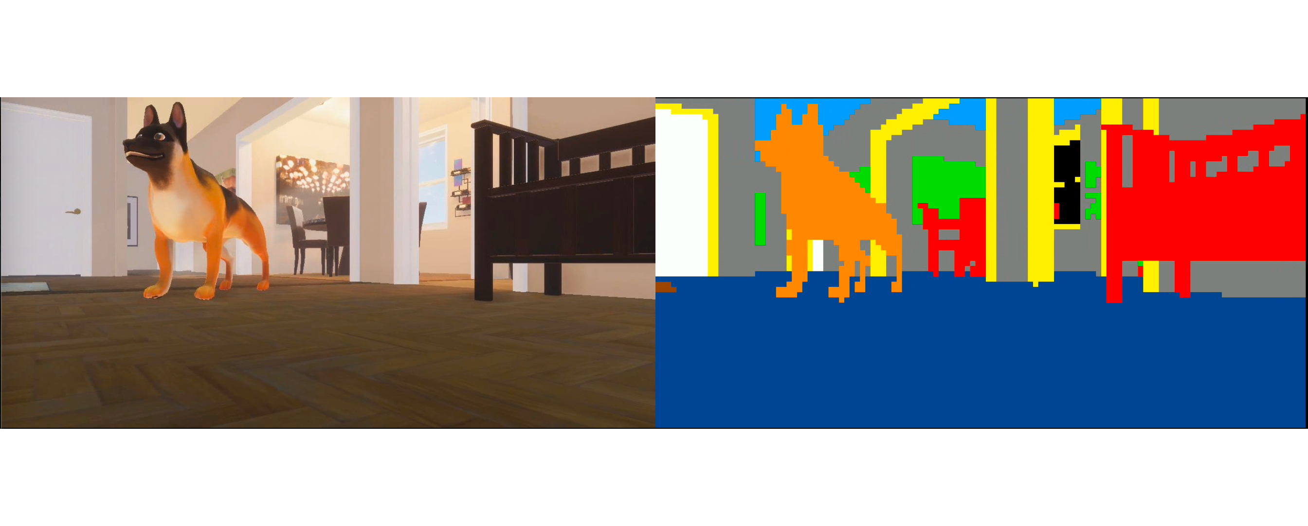
where the colors on the right correspond to the tags that each object in the image carried.

From October to December

The end of the semester was coming quick, and I still hadn’t even trained a neural network yet. As the days got shorter, my work sessions became longer, but school and the cross country season were still getting in the way. Finally Thanksgiving break rolled around, and I had plenty of time to dedicate to this project before the presentation in early December.

Data collection

After some minor lighting improvements and randomization to the first Unity scene, I generated about 10 recordings of the camera moving around to get plenty of data to start with. Then I made another Unity scene with another house environment that I got from the Unity asset store.

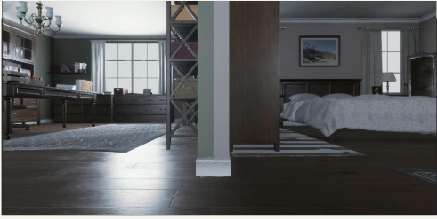
Camera rendition and training data for this scene. The scene itself is simply a line of these rooms, labeled in the same way as the other scene was.

Then, I realized how I could get real world data with labels: image segmentation datasets! Every pixel of images in these datasets are annotated with labels of exactly what kind of object they are. A few quick google searches led me to MIT’s ADE20K image segmentation dataset, and I was able to use their home_and_hotel images to get data from the real world.

For copyright reasons I will not display any of their images here. They do have some examples on their website linked above if you are interested.

Model training

I knew going in that my model would have to be a neural network, since I was working with image data. Very early on I decided against using a CNN, as my patch of pixel size is just 10x10, and a CNN layer would just lose information from already a very small amount of it. I used Tensorflow as my ML backend, since I am already familiar with it.

The neural network I started out with simply consists of three dense layers, and this did end up being the final architecture. The real process of this part of the project was preprocessing the data correctly.

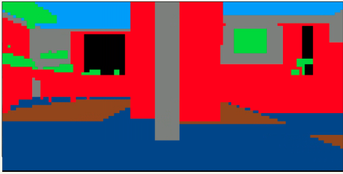
At first I tried just loading all of the data into a tensorflow dataset and feeding it straight into the model. The test images showed that the model seemed to be learning associations:

Tests on the very first model I trained. Notice how it labeled the floor and furniture correctly for the most part, however it barely labeled doorframes (yellow) or “props” (green), which I define as small objects like trash cans, kitchen objects, etc.

I noticed two problems right away. Firstly, the training data is massively skewed simply because most of the area of training images are just walls, furniture or floors, whereas I had defined 6 other categories as well. To combat this I made sure that the dataset contents met quotas for each tag, so that huge skews would not occur.

Secondly, notice how the model labeled the windows and walls in the upper quarter of the image as furniture. Household objects you would call furniture don’t appear on the roof, but the model has no way of building that kind of association with its current inputs. I realized that I could simply include the coordinates of the image input into the model’s training data. I had experimented with Keras models in the past, but this was the first time I had ever fed a model two distinct kinds of information, and I was expecting the model to not handle it well. Thankfully my assumption was wrong.

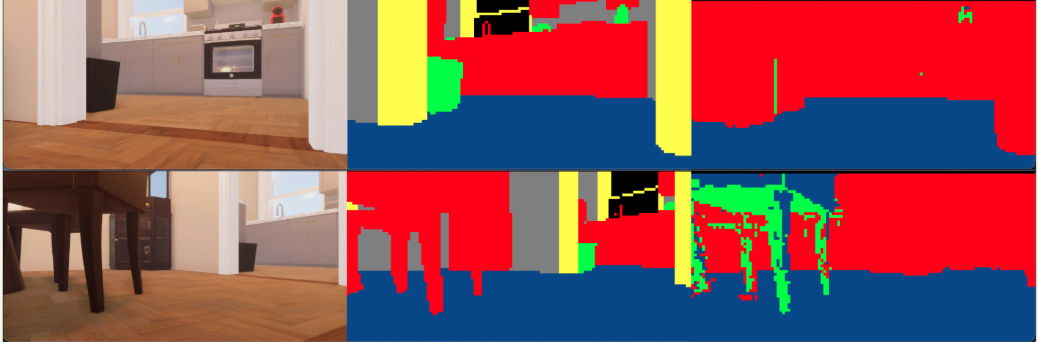
With both of these improvements, my training accuracy jumped from 50% to 76%, and tests on its training data improved. I tested the model on a picture of my house:

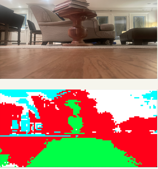
I didn’t really know what I was expecting with this, but I wasn’t let down. The model clearly distinguished between parts of the scene, and accurately labeled all of the furniture. What really bothered me about this test run was the floor: notice how the center part is all labeled differently than the rest, and not even correctly labeled at that.

My next round of improvements included the following:

1. Introducing the ADE20K dataset. I mentioned it in data collection, but it wasn’t actually included in the first datasets. I didn’t see the need for real data until this test.
2. Data augmentation. Since my task is more or less image classification, I took a look at the Image Classification tutorial on Tensorflow’s website for any ideas on improvement, and found the Data Augmentation methods very effective. These are preprocessing layers of the model that randomly brighten, zoom and rotate data before it is sent to the model for training. This is commonly used to help generalize and prevent overfitting, perfect for what I needed to do.
3. Ternary output. Nine categories is a lot for a model to learn, especially when there is lots of data for a few categories and not very much for the rest. I condensed the labels into 3 categories: dynamic, semipermanent, and permanent. I have never actually seen the model make a prediction for semipermanent, so this is effectively a binary output. I labeled only one original category as semipermanent, which is my best guess for why this happens.

After including all of these improvements, I tested the model again on the same image.

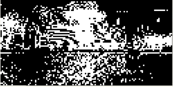
White is dynamic objects, black is permanent.

The model is still confused on the floor, but significantly less so than before. In addition, it accurately labeled most of the rest of the image.

The image above is the last image in my powerpoint that I presented to the judges. The powerpoint is available for download here.

Revisiting it now

I could have made this post in December of 2024 like I promised in part 1, but between finals and college applications it made its way off of my todo list. It found its way back on the list over the winter break, and to compensate for that I wrote a Jupyter notebook that use the pySLAM library to run my algorithm in a visual odometry pipeline. I ran a simple visual odometry pipeline on multiple datasets from the TUM CVG’s RGBD SLAM dataset, once with using my algorithm to filter out features and once not using feature filtering. I calculated the percent improvement in Absolute Trajectory Error (ATE) for each run.

Here are my results:

Model Type	Dataset Name	Control ATE (m)	Experimental ATE (m)	Improvement
All tags	freiburg2_pioneer_slam2	4.474	4.787	-7%
All tags	freiburg3_walking_xyz	0.320	0.306	4%
Ternary	freiburg3_walking_xyz	0.320	0.320	0%
Ternary	freiburg2_pioneer_slam2	4.474	3.519	21%
Ternary	freiburg2_pioneer_slam3	3.864	3.872	0%
Ternary	freiburg2_pioneer_slam	3.886	3.313	15%

It’s no surprise that the model performed the best (relatively) on the SLAM datasets. These were taken by a short household robot which generates images with a view similar to the view of the images in the unity synthetic data. I was surprised to see the 0% improvement of the slam3 dataset, but the results of slam and slam2 more than made up for it.

Final remarks

Despite the all of the time configuring Python ML environments, I enjoyed this project. Using a game engine to generate synthetic data is a fascinating way to get data that otherwise doesn’t exist, and I will surely consider it the next time I am faced with that problem. On a more shallow note, I enjoyed the quick gratification from making small but essential improvements to the training process of the neural network that significantly increased its accuracy.

Of course there are improvements to be made, which are primarily training the model on more varied sources of data. But for now, I will leave this project in a good place.